Boundary-free Scaling Calculations of Laser-Atom Interactions
Z. X. Zhao, B. D. Esry and C. D. Lin
Department of Physics, Kansas State University, Manhattan, Kansas 66506-2601
The most common approaches developed to describe laser-atom interactions are based on sovling the time dependent Schrödinger equation(TDSE) either directly on numerical grids or in a basis set [1]. Neither approaches allow the continuum electrons to escape beyond the boundaries and reflections from these boundaries may result in unphysical interference. Although it is possible to enlarge the box or basis set at a given time step, or by introducing ad hoc absorbers near the boundaries, these approaches are inherently limited. Such limitations can be avoided, however, by adopting a scaled coordinate system, as shown recently by Sidky and Esry [2]. The scaled coordinate is chosen by rescaling the spatial coordinate according to ξ= x/ R(t), where R(t) is set to approach γt at large time t, with γ being an arbitrary velocity. Thus in the scaled coordinate, the electron position does not expand with time.
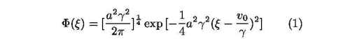
As an illustration in Fig. 1 we show the free propa- gation of a Gaussian wavepacket. The velocity and width of the wavepacket are both 1 a.u. at t=0. The real part of the wavefunctions at t=10 and t=20 are plotted. The solid lines are for the scaled wavefunction and the dotted lines are for the weighted real function R1/2Ψ(Rξ,t). The abscissa is the scaled coordinate ξ, with the scaling paramter R(t) = (1+t2)1/2 for t≥0. At large time the scaled wave function is time independent and is given by
where a and vo are the initial width and velocity, respectively. In this example the center of the wavepacket is located at ξ=1.0 in the scaled coordinate ξ, but the spread of the wavepacket in the real space is large, and the oscillation of Ψ(Rξ,t) is rapid. In the scaled space, on the other hand, the wavefunction is smooth. Examples using scaled coordinates for atoms in an intense laser field will be shown. In the meanwhile, in the scaled coordi- nates the modulus square of the wavefunction also contains information on the ATI peaks directly, see Fig. 2. Here we show how the ATI peaks match the peaks of the density of the wavefunction at the asymptotic time in the scaled space. Details of these calculations will be presented at the conference.
Figures:
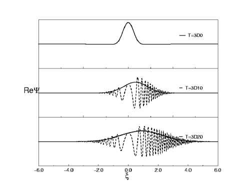
Figure 1: Free propagation of a Gaussian wave packet.
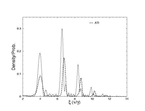
Figure 2:ATI spectrum (dash line) and density plot (solid line). The horizontal
axis is scaled coordinates (or the velocity of electron divided by scaling contant γ).
References:
1) K. Burnett, V. C. Reed and P. L. Knight, J. Phys. B 26, 561 (1993);
M Protopapas, C H Keitel and P. L. Knight, Rep. Prog. Phys. 60 , 389 (1997)
2) E. Y. Sidky and B. D. Esry, Phys. Rev. lett. 85, 5086 (2000)
This work was supported by the
Chemical Sciences, Geosciences and Biosciences Division,
Office of Basic Energy Sciences,
Office of Science,
U.S. Department of Energy.
Submitted to ICPEAC 2001, July 2001 in Santa Fe, NM.
This abstract is also available in Postscript or Adobe Acrobat formats.
|
|